Final Review

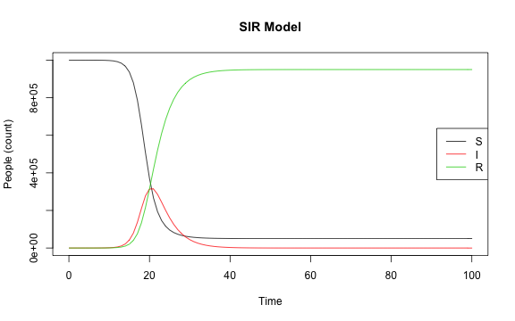
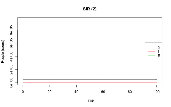
class: center, middle, inverse, title-slide

# Final Review
### Mathew Kiang
### 3/2/2018

---

## Agenda

1. General Tips

1. Reproductive Number

1. Practice exam

1. A tiny bit about deterministic models

1. Open question

---
# Tips

- Know the basic models (e.g., SI, SIR, SIER): when are they appropriate, what are the parameters, what do the parameters mean, how do interventions affect these parameters, etc.

- For SIWR or basic Ross-MacDonald, you should know how to draw and at least roughly know what data you would need to estimate parameters, points of intervention, etc.

- Use the simplest model that you can justify (i.e., don't make age-specific compartments if well-mixed assumption holds, don't make an R compartment if SI will do).

- Remember: heterogeneity is bad. Spatial heterogeneity, network structures, age effects, etc. Compartmental models assume well-mixed populations.

- Probably useful to form groups and just spend an hour going over the quiz and comparing answers. Given how open-ended the quiz was, it is useful to know how other people would address the same question.

---
# Tips

- You will **not** need to know how to calculate `$R_0$` from a model you've never seen before

- You will **not** need to know how to calculate `$R_0$` from given case data

- You will **not** need to know how to code

- You will **not** need to derive anything

---
class: center, middle, inverse
# Reproductive number

---
### What is the reproductive number?

`$R_0$` is "the expected number of secondary cases produced by a typical infected individual early in an epidemic" or "in an entirely susceptible population."

That is, how many people are expected to become infected from a single infectious person in an otherwise susceptible population?

--
### Why is it useful?

Provides a simple threshold:

- If `$R_0 > 1$`, disease is epidemic
- If `$R_0 = 1$`, disease is endemic
- If `$R_0 < 1$`, disease will die out

---

### Basic ( `$R_0$` ) and effective ( `$R_e$` ) reproductive number

#### What if the population is not entirely susceptible?

- Effective reproductive number, `$R_e = R_0 x$` where `$x$` is the proportion of contacts that are susceptible.

#### When do you want one versus the other?

- `$R_0$` will tell you how likely something will spread and its trajectory *early in an epidemic*.

- `$R_e$` will tell you what control measures are necessary to intervene in an endemic situation or later in an epidemic.

---

### How do we calculate `$R_0$`?

--
1. Directly fitting curve to epidemic trajectory
1. From equilibrium values
    - `$R_0 = N/S_{eq}$`
1. From model parameters
    - In a simple SIR, `$$R_0 = \frac{infection}{contact} \times \frac{contacts}{time} \times \frac{time}{infection} = \frac{\beta}{v}=\frac{bk}{v}$$`
    - For more complex models, it is just the rate that people enter the infectious compartment over the rate people leave the infectious compartment (through death, recovery, or some other mechanism)
1. From age of first infection (i.e., higher `$R_0$` results in lower `$A$`)
    - For rectangular age structures, `$R_0 = L/A$`
    - For pyramidal age structures, `$R_0 = 1 + L/A$`
    - Where `$A$` is mean age of (first) infection) and `$L$` is average life span
1. (Also seroprevalence data, but don't use this for final)

---
### When do we need to worry about mortality in estimates?

When in doubt, just calculate both and see what the percent difference is. For example,

`$$R_0 = \frac{bk}{v} \quad \textbf{vs} \quad R_{0}^* = \frac{bk}{v+d}$$`

Where `$v$` is recovery and `$d$` is death rate.

--
### Should you use a fancy method?

No.

### Intuition for age of first infection

A higher `$R_0$` means you have a higher chance of getting infected, which means that your *first* infection is likely to be earlier in life. So for any given life expectancy ($L$), a lower first age of infection ($A$) will result in a higher `$R_0$` in either of the formulas we gave you.

---

class: center, middle, inverse
# Practice exam

## Part A

---
### (1) Incidence vs Prevalence

--
- Incidence is number of *new* cases per unit time.

--
- Prevalence is the fraction of people infected during a specified time period.

### (2) Individual-level risk of disease for infectious vs chronic (non-infectious) diseases

- Infectious disease risk of any individual depends on the status of other individuals. (Not true for chronic (non-infectious) diseases.)

- Thus, there is feedback (infected people infect more people who infect more people) which results in epidemics and incidence occuring over relatively short time scales.

---

### (3) Two ways to measure `$R_0$` at the beginning of an epidemic

1. Fit an exponential curve to the cases at the start and estimate `$R_0$`.

--
1. Use a model to estimate parameters of `$R_0$`.

### (4) Why is measuring `$R_0$` for endemic diseases different? How would you measure it instead?

--
- Population is not entirely susceptible so we cannot use the growth rate of the epidemic.

--
- Measure by estimating age of first infection. (Which formula for which population structure?)

--
- Estimate from `$R_e =R_0 x$` at equilibrium (where `$x$` is proportion of contacts that are susceptible).

---
### (5) What is `$R_e$`? Why do we care?

--
- Average number of secondary infections per infected in a population that is *not* entirely susceptible.

--
- In endemic cases, the population is not entirely susceptible so `$R_0$` may not be as informative.

### (6) Illustrate timelines of acute vs chronic infection. How does quarantine or travel restriction for epidemic containment differ between the two?

--
- Differences between latent, exposure, infectious, and symptomatic periods.

--
- Quarantines are only useful if infectiousness and symptomatic periods overlap.

--
- Travel restrictions can be effective even if infectiousness happens before symptoms.

---
### (7) Pathogen X
--

- (a) Draw it.

- Should have at least SEIAR comparments.

- (b) Write equations

`$$\begin{aligned} \dot{S} &= - \beta S (A + I) + \tau R \\
\dot{E} &= \beta S(A+I) - \gamma E - \delta E \\
\dot{I} &= \gamma E - \rho I \\
\dot{A} &= \delta E - \sigma A \\
\dot{R} &= \sigma A + \rho I - \tau R \end{aligned}$$`

- (c) Name 2 types of heterogeneity

- Contact, age, spatial, disease progression, etc.

---
### (8) Why is vector control effective (according to R-M model)?

`$$R_0 = \frac{ma^2bce^{-\mu T}}{r\mu}$$`

- Mosquito-related terms have a disproportionate effect (e.g., `$a$` is squared, `$\mu$` is both the exponent and in the denominator, etc.).

- Punchline of the paper is that the incubation period is close to the lifespan of the mosquito so if you shorten the lifespan a little, it'll never incubate.

---
class: center, middle, inverse

# Practice exam

## Part B

---
### (1) CFR and concerns?

- CFR = 20/112

- Concerns: asymptomatics, diagnosis in general, reporting rates, etc.

### (2) Cholera Model and contact parameter

- Draw it.

- Cholera has an environmental reservoir so we must figure out contribution to and access of shared water sources.

---

### (3) SIW initial analysis

- Useful because initial `$R_0$` estimates could give policymakers an idea of trajectory and likely spread of the disease.

### (4) SIW and difficulties

- Contact with water supply is hard to meaasure.

- Contributions of infectious people to the reservoir is hard to parameterize.

- Dynamics of vibrios in the water is hard to measure.

- Population at risk is often hard (e.g., what is the total volume of water in the reservoir?)

---
### (5) Fraction to vaccinate

- `$P = 1 - \frac{1}{R_0}$`

### (6) Defining "at-risk"

- Hard to define access to water in general (especially in low-income settings)

- Hard to define spatial/social perimeters of random mixing models

### (7) Effect of implementation time

- If epidemic is highly localized and implementation takes as long as the epidemic lasts, then it's not useful or might have already moved on to other areas.

---
### (8) Spatial extensions? Mobility?

- Agent-based modeling or metapopulation models where you incorporate mobility as a force of infection parameter.

- **You do not need to know how to do this or write the equations**. You just need to know it exists.

### (9) Agent-based models vs math model

- ABMs allow you to incorporate individual or spatial heterogeneity more easily and keep track of individual status (e.g., vaccines).

- Much more detail and flexibility in ABMS.

- Less transparent, harder interpretation, computationally more difficult.

---

# Deterministic Models

- Let's pretend I run an SIR model with `$\beta = 0.35$`, `$k = 4$`, and `$r = 0.333$` to equilibrium. This is the plot:

![](index_files/figure-html/unnamed-chunk-1-1.png)

---

# Deterministic Models

- At equilibrium (after 300 days), the final values of the compartments were:

```r
simulation[nrow(simulation), ]
```

```
##     time     S         I      R
## 101  100 50014 0.0001366 949986
```

- If I take these final values (at equilbrium) and I put them in a new simulation as my *initial values*, what will happen? What will the plot look like?

```r
new_inits <- c(S = simulation[nrow(simulation), "S"], 
               I = simulation[nrow(simulation), "I"], 
               R = simulation[nrow(simulation), "R"])
simulation2 <- as.data.frame(ode(y = new_inits, 
                                 times = dt, 
                                 func = SIR, parms = parms))
```

---

# Deterministic Models

```r
matplot(x = simulation2[, 1], y = simulation2[, 2:4], type = "l", 
        lty = 1, xlab = "Time", ylab = "People (count)", main = "SIR (2)")
legend(x = "right", legend = c('S', 'I', 'R'), col = 1:3, lty = 1)
```

![](index_files/figure-html/unnamed-chunk-4-1.png)

---
class: center, middle, inverse
# You're going to be fine