Measles Worksheet

class: center, middle, inverse, title-slide

# Measles Worksheet
## From 1/30 lecture – But Slower
### Mathew Kiang
### 1/31/2017

---

# Goals for today

1. Go over the measles handout

- Sort of. Not going to answer the questions for you. Just going to help you go through the code to answer them on your own.

---
class: center, middle, inverse
# Question 1
## Make an SIR model for measles

---
## Question 1

- Measles epidemic: 
    - Population: 1 million
    - Probability of infection is `$.75$` if in contact with an infectious person
    - 12 respiratory contacts **per week**
    - Disease duration of 1 week
    - For now, use SIR framework

---

```r
library(deSolve)

parms <- c(beta = 0.333, k = 3 , r = 0.333)
inits <- c(S = 499, I = 1, R = 0)
dt <- seq(0, 300, 1)

SIR <- function(t, x, parms){
    with(as.list(c(parms, x)), {
    
        N <- S + I + R
        dS <- - (beta * k * S * I) / N
        dI <- + (beta * k * S * I) / N - r * I
        dR <- r * I

der <- c(dS, dI, dR)
    
        return(list(der))
    }) 
}

simulation <- as.data.frame(ode(y = inits, times = dt, 
                                func = SIR, parms = parms))
```
Start with the boilerplate code we gave you last week.
---

```r
library(deSolve)

*parms <- c(beta = 0.333, k = 3 , r = 0.333)
*inits <- c(S = 499, I = 1, R = 0)
*dt <- seq(0, 300, 1)

SIR <- function(t, x, parms){
    with(as.list(c(parms, x)), {
    
        N <- S + I + R
        dS <- - (beta * k * S * I) / N
        dI <- + (beta * k * S * I) / N - r * I
        dR <- r * I

der <- c(dS, dI, dR)
    
        return(list(der))
    }) 
}

simulation <- as.data.frame(ode(y = inits, times = dt,
                                func = SIR, parms = parms))
```
Modify the parameters we were given.

---

```r
library(deSolve)

*parms <- c(beta = 0.75, k = 12 , r = 1)
*inits <- c(S = 999999, I = 1, R = 0)
dt <- seq(0, 300, 1)

SIR <- function(t, x, parms){
    with(as.list(c(parms, x)), {
    
        N <- S + I + R
        dS <- - (beta * k * S * I) / N
        dI <- + (beta * k * S * I) / N - r * I
        dR <- r * I

der <- c(dS, dI, dR)
    
        return(list(der))
    }) 
}

simulation <- as.data.frame(ode(y = inits, times = dt,
                                func = SIR, parms = parms))
```
Modify the parameters we were given.

- 12 contacts per week
- disease duration is 1 week
- .75 probability of infectiousness
- 1 million people in the population

---

```r
library(deSolve)

parms <- c(beta = 0.75, k = 12 , r = 1)
inits <- c(S = 999999, I = 1, R = 0)
*dt <- seq(0, 10, 1/7)

SIR <- function(t, x, parms){
    with(as.list(c(parms, x)), {
    
        N <- S + I + R
        dS <- - (beta * k * S * I) / N
        dI <- + (beta * k * S * I) / N - r * I
        dR <- r * I

der <- c(dS, dI, dR)
    
        return(list(der))
    }) 
}

simulation <- as.data.frame(ode(y = inits, times = dt,
                                func = SIR, parms = parms))
```
Make sure your time scale makes sense given your parameters.

- 300 weeks seems too long, so we change it to 10 weeks.
- 1 week at a time is too coarse, so we change it to days (`$\frac{1}{7}$`)
--

- But **any** small number would work

---

```r
matplot(x = simulation[, 1], y = simulation[, 2:4], type = "l", 
        lty = 1, xlab = "Time (weeks)", ylab = "People (count)", 
        main = "Measles")
legend(x = "right", legend = c('S', 'I', 'R'), 
       col = 1:3, lty = 1)
```

![](index_files/figure-html/unnamed-chunk-5-1.png)
---
class: center, middle, inverse
# Time-steps are arbitrary
## For example, let's do days
---

```r
*parms <- c(beta = 0.75, k = 12/7 , r = 1/7)
inits <- c(S = 999999, I = 1, R = 0)
*dt <- seq(0, 10 * 7, 1)

simulation_days <- as.data.frame(ode(y = inits, times = dt,
                                     func = SIR, parms = parms))
```
- Since our `parms` are in units of weeks, we divide by `$7$` to make them days

- We change our time-steps to be 70 units of 1 day to match our previous simulation
--

- **NOTE:** We save the simulations in different variable

- How will the plot change?

---

```r
matplot(x = simulation_days[, 1], y = simulation_days[, 2:4], type = "l", 
        lty = 1, xlab = "Time (days)", ylab = "People (count)", 
        main = "Measles")
legend(x = "right", legend = c('S', 'I', 'R'), 
       col = 1:3, lty = 1)
```

![](index_files/figure-html/unnamed-chunk-7-1.png)
The plot does not change. 
---
We can verify this by looking directly at the data.

```r
head(simulation)
```

```
##     time      S       I      R
## 1 0.0000 999999   1.000  0.000
## 2 0.1429 999997   3.136  0.267
## 3 0.2857 999989   9.833  1.104
## 4 0.4286 999965  30.832  3.729
## 5 0.5714 999891  96.671 11.960
## 6 0.7143 999659 303.054 37.764
```

```r
head(simulation_days)
```

```
##   time      S       I      R
## 1    0 999999   1.000  0.000
## 2    1 999997   3.136  0.267
## 3    2 999989   9.833  1.104
## 4    3 999965  30.832  3.729
## 5    4 999891  96.671 11.960
## 6    5 999659 303.054 37.764
```
The top is in weeks, the bottom is in days.
---
class: center, middle, inverse
# Do this for chickenpox (b=.51) 
# and then mumps (b=.38).red[*]
## (You can do this on your own — I believe in you.)
.footnote[.red[*] Don't forget to save the results in different variables.]
---
# Hopefully, your code looks like this:

```r
parms_mumps <- c(beta = 0.38, k = 12 , r = 1)
parms_cpox <- c(beta = .51, k = 12, r = 1)
sim_mumps <- as.data.frame(ode(y = inits, times = dt,
                               func = SIR, parms = parms_mumps))
sim_cpox <- as.data.frame(ode(y = inits, times = dt,
                               func = SIR, parms = parms_cpox))
```
- Just make a new set of `parms` for each disease

- Change the parameter as appropriate

- Run the new simulations and save the results in new variables

- `dt` didn't change, our model (`SIR()`) didn't change, and `inits` didn't change.
---
class: center, middle, inverse
# How to plot multiple things
## For example, to compare infectious curves
---
# Compare multiple infectious curves

![](index_files/figure-html/unnamed-chunk-11-1.png)
---
# Wait, what?

```r
*plot(x = simulation$time, y = simulation$I, type = "l",
*    xlab = "Time (weeks)", ylab = "People (count)", main = "Infections")
lines(x = sim_cpox$time, y = sim_cpox$I, col = "red")
lines(x = sim_mumps$time, y = sim_mumps$I, col = "green")
legend(x = "topright", legend = c('Measles', 'Chicken Pox', 'Mumps'), 
       col = c("black", "red", "green"), lty = 1)
```
- Plot one of the curves (see last week's slides or `help(plot)`) for more.
    - `type = 'l'` means you want a `l`ine.
    - `xlab`, `ylab`, and `main` are the x-axis, y-axis, and main labels, respectively.
---
# Wait, what?

```r
plot(x = simulation$time, y = simulation$I, type = "l",
    xlab = "Time (weeks)", ylab = "People (count)", main = "Infections")
*lines(x = sim_cpox$time, y = sim_cpox$I, col = "red")
lines(x = sim_mumps$time, y = sim_mumps$I, col = "green")
legend(x = "topright", legend = c('Measles', 'Chicken Pox', 'Mumps'), 
       col = c("black", "red", "green"), lty = 1)
```
- Plot one of the curves (see last week's slides or `help(plot)`) for more.
    - `type = 'l'` means you want a `l`ine.
    - `xlab`, `ylab`, and `main` are the x-axis, y-axis, and main labels, respectively.
- Now plot a second curve, using `lines()` — make sure to give it a different color. 
    - Recall you use `lines()` to **add** to an existing `plot()` object.
---
# Wait, what?

```r
plot(x = simulation$time, y = simulation$I, type = "l",
    xlab = "Time (weeks)", ylab = "People (count)", main = "Infections")
lines(x = sim_cpox$time, y = sim_cpox$I, col = "red")
lines(x = sim_mumps$time, y = sim_mumps$I, col = "green")
*legend(x = "topright", legend = c('Measles', 'Chicken Pox', 'Mumps'), 
*      col = c("black", "red", "green"), lty = 1)
```
- Plot one of the curves (see last week's slides or `help(plot)`) for more.
    - `type = 'l'` means you want a `l`ine.
    - `xlab`, `ylab`, and `main` are the x-axis, y-axis, and main labels, respectively.
- Now plot a second curve, using `lines()` — make sure to give it a different color. 
    - Recall you use `lines()` to **add** to an existing `plot()` object.
- Add the third curve — again, make sure to give it a different color.
- Add a legend, specifying each line in order under `legend` and each color in order under `col`.
---
class: center, middle, inverse
# How to find the time of max infections
## Also, how to use max()
---
# When was the peak of infections?
We could just eyeball it, but instead, let's find the value of our `time` column when the peak of the **measles** epidemic occurred.
--

```r
simulation$time[which.max(simulation$I)]
```

```
## [1] 2
```
--

So the epidemic occurred at exactly two weeks — aggreeing with our plot.

---

# Ok, what's happening?

```r
simulation$time[which.max(simulation$I)]
```
- `which.max()` is a function that returns the index (location) of the maximum value in a vector

- `$` is shorthand for specifying a single column

- `[ ]` is shorthand for selecting a specific subset

- So we are saying "find the row index that corresponds to the highest value of `simulation$I`"

- Now take that row index and return the corresponding value of `simulation$time`

---
# Let's verify
Find the maximum value of `simulation$I`:
--

```r
max(simulation$I)
```

```
## [1] 644530
```
--
Which index is this max value? (`TRUE` means we hit the max, `FALSE` otherwise)

```r
max(simulation$I) == simulation$I
```

```
##  [1] FALSE FALSE FALSE FALSE FALSE FALSE FALSE FALSE FALSE FALSE FALSE
## [12] FALSE FALSE FALSE  TRUE FALSE FALSE FALSE FALSE FALSE FALSE FALSE
## [23] FALSE FALSE FALSE FALSE FALSE FALSE FALSE FALSE FALSE FALSE FALSE
## [34] FALSE FALSE FALSE FALSE FALSE FALSE FALSE FALSE FALSE FALSE FALSE
## [45] FALSE FALSE FALSE FALSE FALSE FALSE FALSE FALSE FALSE FALSE FALSE
## [56] FALSE FALSE FALSE FALSE FALSE FALSE FALSE FALSE FALSE FALSE FALSE
## [67] FALSE FALSE FALSE FALSE FALSE
```
Note here that the only `TRUE` is in the 15th position.
---
# Let's verify
So we could just ask for the 15th row of `simulation$time`:
--

```r
simulation$time[15]     ## equiv: simulation[15, 'time']
```

```
## [1] 2
```
--
Or we could just pass the entire boolean vector:

```r
simulation$time[max(simulation$I) == simulation$I]
```

```
## [1] 2
```
--
Or better yet, just stick to `which.max()`
---
# Aside: Boolean vectors

Just a vector of `TRUE` or `FALSE` (or `NA`) for whatever condition you specify.

Always equal to the length of the vector being compared.

What does this return? (Recall what `seq()` does from our last lab)

```r
seq(-5, 5, 1) >= 0
```
--

- How long will the return vector be?
- How many `FALSE`? 
- How many `TRUE`?
--

```r
print(seq(-5, 5, 1) >= 0)
```

```
##  [1] FALSE FALSE FALSE FALSE FALSE  TRUE  TRUE  TRUE  TRUE  TRUE  TRUE
```
---
class: center, middle, inverse
# Use one of these methods to find
# the time of maximum infection for
# mumps and chickenpox.red[*]
.footnote[.red[*] Just use `which.max()`.]
---
# Answers

```r
simulation$time[which.max(simulation$I)]
```

```
## [1] 2
```

```r
sim_mumps$time[which.max(sim_mumps$I)]
```

```
## [1] 4
```

```r
sim_cpox$time[which.max(sim_cpox$I)]
```

```
## [1] 3
```
**NOTE:** My answers will be rounded. Yours should not be.
---
class: center, middle, inverse
# Find the peak number of infected for each of the three epidemics
---
# Answers

```r
max(simulation$I)
```

```
## [1] 644530
```

```r
max(sim_mumps$I)
```

```
## [1] 405947
```

```r
max(sim_cpox$I)
```

```
## [1] 537860
```
---
class: center, middle, inverse
# Question 4
## SEIR Models
---
class: center, middle
# Write out an SEIR model
## With parameter a for the rate from latent to infectious
---
class: center, middle
# Seriously, write it out
## Always write/draw models before coding them
---

```r
parms <- c(beta = .75, k = 12 , r = 1)
inits <- c(S = 999999, I = 1, R = 0)
dt <- seq(0, 10, 1/7)

SIR <- function(t, x, parms){
    with(as.list(c(parms, x)), {
    
        N <- S + I + R
        dS <- - (beta * k * S * I) / N
        dI <- + (beta * k * S * I) / N - r * I
        dR <- r * I

der <- c(dS, dI, dR)
    
        return(list(der))
    }) 
}

simulation <- as.data.frame(ode(y = inits, times = dt, 
                                func = SIR, parms = parms))
```
Start with the boilerplate code again
---

```r
*parms <- c(beta = .75, a = 1/12 * 7, k = 12 , r = 1)
inits <- c(S = 999999, E =0, I = 1, R = 0)
dt <- seq(0, 10, 1/7)

SIR <- function(t, x, parms){
    with(as.list(c(parms, x)), {
    
        N <- S + I + R
        dS <- - (beta * k * S * I) / N
        dI <- + (beta * k * S * I) / N - r * I
        dR <- r * I

der <- c(dS, dI, dR)
    
        return(list(der))
    }) 
}

simulation <- as.data.frame(ode(y = inits, times = dt, 
                                func = SIR, parms = parms))
```
- Introduce a new parameter `a` be the rate from latent to infectious.
--

- If the duration of the latent period is 12 days, what is the rate per day?

--
**1/12**

--
    - Note, we want the rate to be per week (since our time-steps are in weeks) so `* 7`
---

```r
parms <- c(beta = .75, a = 1/12 * 7, k = 12 , r = 1)
*inits <- c(S = 999999, E =0, I = 1, R = 0) 
*dt <- seq(0, 25, 1/7)

SIR <- function(t, x, parms){
    with(as.list(c(parms, x)), {
    
        N <- S + I + R
        dS <- - (beta * k * S * I) / N
        dI <- + (beta * k * S * I) / N - r * I
        dR <- r * I

der <- c(dS, dI, dR)
    
        return(list(der))
    }) 
}

simulation <- as.data.frame(ode(y = inits, times = dt, 
                                func = SIR, parms = parms))
```
- Need to add an initial value for our new compartment `E`

- Also, intuitively, delaying infectiousness will delay the epidemic so we should expand our time
---

```r
parms <- c(beta = .75, a = 1/12 * 7, k = 12 , r = 1)
inits <- c(S = 999999, E =0, I = 1, R = 0)
dt <- seq(0, 25, 1/7)

*SEIR <- function(t, x, parms){
    with(as.list(c(parms, x)), {
    
        N <- S + I + R
        dS <- - (beta * k * S * I) / N
        dI <- + (beta * k * S * I) / N - r * I
        dR <- r * I

der <- c(dS, dI, dR)
    
        return(list(der))
    }) 
}

simulation <- as.data.frame(ode(y = inits, times = dt, 
                                func = SIR, parms = parms))
```
Change the function name to reflect our new model
---

```r
parms <- c(beta = .75, a = 1/12 * 7, k = 12 , r = 1)
inits <- c(S = 999999, E =0, I = 1, R = 0)
dt <- seq(0, 25, 1/7)

SEIR <- function(t, x, parms){
    with(as.list(c(parms, x)), {
    
*       N <- S + E + I + R 
        dS <- - (beta * k * S * I) / N
*       dE <- + (beta * k * S * I) / N - (a * E)
        dI <- + (a * E) - (r * I)
        dR <- r * I

der <- c(dS, dI, dR)
    
        return(list(der))
    }) 
}

simulation <- as.data.frame(ode(y = inits, times = dt, 
                                func = SIR, parms = parms))
```
Add `E` into our total population count `N` and then put in the compartment
---

```r
parms <- c(beta = .75, a = 1/12 * 7, k = 12 , r = 1)
inits <- c(S = 999999, E =0, I = 1, R = 0)
dt <- seq(0, 25, 1/7)

SEIR <- function(t, x, parms){
    with(as.list(c(parms, x)), {
    
        N <- S + E + I + R 
        dS <- - (beta * k * S * I) / N
        dE <- + (beta * k * S * I) / N - (a * E)
*       dI <- + (a * E) - (r * I)
        dR <- r * I

*       der <- c(dS, dE, dI, dR) 
    
        return(list(der))
    }) 
}

simulation <- as.data.frame(ode(y = inits, times = dt, 
                                func = SIR, parms = parms))
```
Adjust the `I` compartment since things can only come from `E` now.

Don't forget to return the `dE` compartment.
---

```r
parms <- c(beta = .75, a = 1/12 * 7, k = 12 , r = 1)
inits <- c(S = 999999, E =0, I = 1, R = 0)
dt <- seq(0, 25, 1/7)

SEIR <- function(t, x, parms){
    with(as.list(c(parms, x)), {
    
        N <- S + E + I + R 
        dS <- - (beta * k * S * I) / N
        dE <- + (beta * k * S * I) / N - (a * E)
        dI <- + (a * E) - (r * I)
        dR <- r * I

der <- c(dS, dE, dI, dR)
    
        return(list(der))
    }) 
}

*sim_seir <- as.data.frame(ode(y = inits, times = dt, 
*                             func = SEIR, parms = parms))
```
Save it into a new variable and make sure to use the correct model.
---
# Plot should look like this

```r
sim_seir <- as.data.frame(ode(y = inits, times = dt, 
                              func = SEIR, parms = parms))
matplot(x = sim_seir[, 1], y = sim_seir[, 2:5], type = "l", 
        lty = 1, xlab = "Time", ylab = "People (count)", main = "SEIR Model")
legend(x = "right", legend = c('S', 'E', 'I', 'R'), col = 1:4, lty = 1)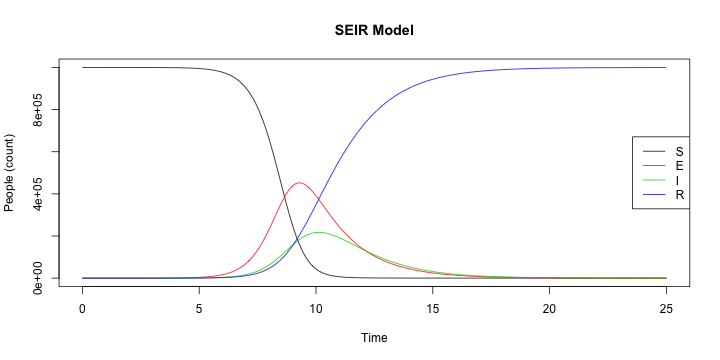
```

![](index_files/figure-html/unnamed-chunk-34-1.png)
---
class: center, middle, inverse
# With a neighbor, add births/deaths to your SEIR model
## You can only be born S but you can die in any compartment.red[*]

.footnote[.red[*]Keep births and deaths equal assuming an annual fertility and mortality rate of .02]
---
# Your code should look similar

```r
# added births and deaths as weekly rates (divide by 52 weeks)
parms_bd <- c(beta = .75, a = 1/12 * 7, k = 12 , r = 1, 
              b = .02/52, d = .02/52)
# Look at 50 years
dt_bd <- seq(0, 52 * 50, 1/7)

SEIR_bd <- function(t, x, parms){
    with(as.list(c(parms, x)), {
    
        N <- S + E + I + R 
        dS <- - (beta * k * S * I) / N + (b * N) - (d * S)
        dE <- + (beta * k * S * I) / N - (a * E) - (d * E)
        dI <- + (a * E) - (r * I) - (d * I)
        dR <- r * I  - (d * R)

der <- c(dS, dE, dI, dR)
    
        return(list(der))
    }) 
}
simulation_bd <- as.data.frame(ode(y = inits, times = dt_bd, 
                                   func = SEIR_bd, parms = parms_bd))
```
---
# Your plot should look like this

```r
matplot(x = simulation_bd[, 1], y = simulation_bd[, 2:5], type = "l", 
        lty = 1, xlab = "Time", ylab = "People (count)", 
        main = "SEIR with births/deaths")
legend(x = "right", legend = c('S', 'E', 'I', 'R'), col = 1:4, lty = 1)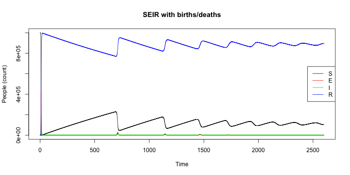
```

![](index_files/figure-html/unnamed-chunk-36-1.png)
---
class: center, middle, inverse
# Challenge questions
## See if you can reparaterize the same model, but in time steps of years.
---
class: center, middle, inverse
# Question 5
## With a neighbor, plot only infected individuals 
## (and only for t > 5 years)
---
# Hints
--

### We went over all the code you need to do this

--
### Boolean vectors are your friend

--
### How you parameterized time matters

---
# Your plot should look like this

```r
plot(x = simulation_bd$time[simulation_bd$time >= 5 * 52], 
     y = simulation_bd$I[simulation_bd$time >= 5 * 52], 
     type = "l", lty = 1, xlab = "Time", ylab = "Infections (count)", 
     main = "Infections, Open SEIR")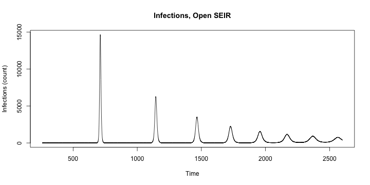
```

![](index_files/figure-html/unnamed-chunk-37-1.png)
---
# Or save the vector

```r
y5_higher <- simulation_bd$time >= 5 * 52
plot(x = simulation_bd$time[y5_higher], 
     y = simulation_bd$I[y5_higher], 
     type = "l", lty = 1, xlab = "Time", ylab = "Infections (count)", 
     main = "Infections, Open SEIR")
```

![](index_files/figure-html/unnamed-chunk-38-1.png)
---
class: center, middle, inverse
# Question 6
## What the for-loop?
## (The magic of not copying and pasting)
---
# For-loop basics
Suppose you want to sweep through many values of a parameter.

You could just do this:

```r
parms_bd1 <- c(beta = .75, a = 1/12 * 7, k = 12 , r = 1, 
              b = .020/52, d = .020/52)
parms_bd1 <- c(beta = .75, a = 1/12 * 7, k = 12 , r = 1, 
              b = .025/52, d = .025/52)
parms_bd1 <- c(beta = .75, a = 1/12 * 7, k = 12 , r = 1, 
              b = .030/52, d = .030/52)
parms_bd1 <- c(beta = .75, a = 1/12 * 7, k = 12 , r = 1, 
              b = .035/52, d = .035/52)
```
--

But that's error-prone, tedious, and ugly.

So we're going to use a loop.
---
# For-loop basics
## The anatomy of a for loop

```r
for (placeholder_variable in list_of_values) {
    ## Do something -- hopefully more useful than printing
    print(placeholder_variable)
}
```
---
# For-loop basics
## The anatomy of a for loop

```r
*for (placeholder_variable in list_of_values) {
    ## Do something -- hopefully more useful than printing
    print(placeholder_variable)
}
```
- `for()` declares you are going to make a loop in the `{`brackets`}`
- To use `for()` we need to give it something to loop through — `list_of_values`
---
# For-loop basics
## The anatomy of a for loop

```r
for (placeholder_variable in list_of_values) {
    ## Do something -- hopefully more useful than printing
*   print(placeholder_variable)
}
```
- `for()` declares you are going to make a loop in the `{`brackets`}`
- To use `for()` we need to give it something to loop through — `list_of_values`
- We also need to give it a `placeholder_variable` we will use to refer to the current value from `list_of_values` inside of the `{`brackets`}`.
- Finally, we do something to that `placeholder_variable` and then move on to the next value
---
# For-loop basics
## The anatomy of a for loop

```r
sentence <- c("The", "magic", "of", "for", "loops")
for (word in sentence) {
    ## Do something -- hopefully more useful than printing
    print(word)
}
```

```
## [1] "The"
## [1] "magic"
## [1] "of"
## [1] "for"
## [1] "loops"
```
--
So the first time this loop ran, `word` had the value of "The"

The second time, `word` had the value of "magic" and so on.

---
# For-loop basics
## Sidenote, you can also loop by index

```r
sentence <- c("The", "magic", "of", "for", "loops")
for (idx in 1:5) {
    ## Do something -- hopefully more useful than printing
    print(sentence[idx])
}
```

```
## [1] "The"
## [1] "magic"
## [1] "of"
## [1] "for"
## [1] "loops"
```

Very common because it is more general

Useful when you only care about the position of an element (and not the element itself).
---
# For-loop basics
## Appending data with loops

```r
multiplier <- 1:5
holder <- NULL
for (x in multiplier) {
    results <- 1:10 * x
    holder <- cbind(holder, results)
}
```
What is this code doing?
---
# For-loop basics
## Appending data with loops

```r
*multiplier <- 1:5
holder <- NULL
for (x in multiplier) {
    results <- 1:10 * x
    holder <- cbind(holder, results)
}
```
What is this code doing?

- `multiplier` is just a sequence `1, 2, 3, 4, 5`
---
# For-loop basics
## Appending data with loops

```r
multiplier <- 1:5
*holder <- NULL
for (x in multiplier) {
    results <- 1:10 * x
    holder <- cbind(holder, results)
}
```
What is this code doing?

- `multiplier` is just a sequence `1, 2, 3, 4, 5`

- Variables inside the `{`brackets`}` of the `for` loop get overwritten with every loop, so we create an empty (`NULL`) variable **outside** of the `for` loop to store results.
---
# For-loop basics
## Appending data with loops

```r
multiplier <- 1:5
holder <- NULL
for (x in multiplier) {
    results <- 1:10 * x
*    holder <- cbind(holder, results)
}
```
What is this code doing?

- `multiplier` is just a sequence `1, 2, 3, 4, 5`

- Variables inside the `{`brackets`}` of the `for` loop get overwritten with every loop, so we create an empty (`NULL`) variable **outside** of the `for` loop to store results.

- Then we `c`olumn `bind` our inside-the-loop results to the outside-the-loop variable we made
---
# For-loop basics
## Appending data with loops

```r
print(holder)
```

```
##       results results results results results
##  [1,]       1       2       3       4       5
##  [2,]       2       4       6       8      10
##  [3,]       3       6       9      12      15
##  [4,]       4       8      12      16      20
##  [5,]       5      10      15      20      25
##  [6,]       6      12      18      24      30
##  [7,]       7      14      21      28      35
##  [8,]       8      16      24      32      40
##  [9,]       9      18      27      36      45
## [10,]      10      20      30      40      50
```
---
class: center, middle, inverse
# Back to Question 6
## With a neighbor, make a vector containing 5 equally spaced values of the birth/death parameter between .013 and .025..red[*]

.footnote[.red[*]See `help(seq)` for options]
---
class: center, middle, inverse
# Back to Question 6
## Now make a for loop that runs ode on each value of this vector and use the "appending trick" to save **only** the infectious column from each run into a new variable.red[*]

.footnote[.red[*]Change your time scale to 25 years instead of 50]
---
class: center, middle, inverse
# Back to Question 6
## Now plot your five infectious columns 
## for time >= 5 years
---
# Changing birth/death rates

```r
bd_rates <- seq(from = .013, to = .025, length.out = 5)
dt_bd <- seq(0, 25 * 52, 1/7)
holder <- NULL
for (bd in bd_rates) {
    parms_bd <- c(beta = .75, a = 1/12 * 7, k = 12 , r = 1, 
                  b = bd/52, d = bd/52)
    simulation_bd <- as.data.frame(ode(y = inits, times = dt_bd, 
                                       func = SEIR_bd, parms = parms_bd))
    holder <- cbind(holder, simulation_bd$I)
}
```
Nothing on this slide is new. We're just piecing together different things we've done before. Review it slowly if it doesn't make sense to you yet.
---
# Changing birth/death rates

```r
t5_more <- simulation_bd$time >= 52 * 5
matplot(simulation_bd$time[t5_more], holder[t5_more, ], type = 'l', 
        lty = 1, xlab = "Time (weeks)", ylab = "Infections (count)", 
        main = "Changing birth/deaths")
legend(x = "topleft", legend = bd_rates, col = 1:5, lty = 1)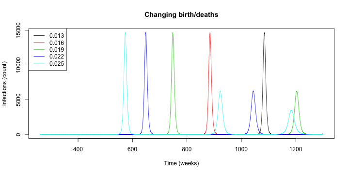
```

![](index_files/figure-html/unnamed-chunk-53-1.png)

---
class: center, middle, inverse
# That's it.
## Thanks