Age-standardized synthetic-opioid death rates by sex

This vignette turns multiple-cause-of-death (MCOD) records into an age-standardized synthetic-opioid death rate by sex, for US residents only, illustrated with 1999, 2010, and 2020. Synthetic opioids other than methadone are ICD-10 T40.4, flagged by flag_opioid_types() as other_synth_present. T40.4 is the CDC-standard proxy for illicitly manufactured fentanyl, but it is a proxy – it also captures tramadol, U-47700, and other synthetics. Its composition shifts over time: illicit fentanyl only came to dominate T40.4 around 2013-2014 (Ciccarone’s “third wave”), so early-series T40.4 deaths are largely pharmaceutical fentanyl and tramadol, not the illicit-fentanyl phenomenon of recent years. Read a long T40.4 series as “synthetic opioids,” not “fentanyl,” throughout. Denominators are the SEER bridged-race estimates (race_scheme = "bridged"), one internally consistent race series, so the comparison is not confounded by a change in how the Census classifies people by race.

All death data below are small inline synthetic counts, clearly labelled illustrative; only the bundled population denominators are real. No chunk reads a restricted record, an external file, or the network.

This vignette picks up where flagging leaves off. The Classifying overdose deaths vignette (vignette("classifying-overdose-deaths")) builds the drug_death/opioid_death flags used here and is the place to start if the flag steps below are unfamiliar. For the full record-to-analysis workflow, begin with vignette("getting-started").

library(narcan)

From records to a fentanyl flag

Start with a handful of illustrative record-level rows. Real MCOD data carry restatus (residency) and ucod (underlying cause) as raw columns, plus a derived f_records_all – the space-joined multiple-cause T-code string that the flag helpers key on (f_records_all is produced by unite_records(); see vignette("getting-started")).

records <- data.frame(
    year          = 2020L,
    restatus      = c(1L, 1L, 4L, 2L, 3L),
    ucod          = c("X42", "X44", "X42", "I250", "X42"),
    f_records_all = c("T404 T519", "T404", "T404", "I250", "T400"),
    age           = c(35L, 40L, 55L, 60L, 25L),
    sex           = c("male", "female", "male", "male", "female"),
    stringsAsFactors = FALSE
)
records
#>   year restatus ucod f_records_all age    sex
#> 1 2020        1  X42     T404 T519  35   male
#> 2 2020        1  X44          T404  40 female
#> 3 2020        4  X42          T404  55   male
#> 4 2020        2 I250          I250  60   male
#> 5 2020        3  X42          T400  25 female

subset_residents() keeps restatus %in% 1:3 and drops the column. The non-resident row (restatus == 4) is removed.

resid <- subset_residents(records)
resid
#>   year ucod f_records_all age    sex
#> 1 2020  X42     T404 T519  35   male
#> 2 2020  X44          T404  40 female
#> 3 2020 I250          I250  60   male
#> 4 2020  X42          T400  25 female

flag_drug_deaths() adds drug_death under the ISW7 (Injury Surveillance Workgroup) rule – a drug ucod and a T-code. The cardiac death (I250) is not a drug death.

resid <- flag_drug_deaths(resid, year = 2020)
resid[, c("ucod", "f_records_all", "drug_death")]
#>   ucod f_records_all drug_death
#> 1  X42     T404 T519          1
#> 2  X44          T404          1
#> 3 I250          I250          0
#> 4  X42          T400          1

flag_opioid_deaths() adds opioid_death. flag_opioid_types() then splits the opioid into type flags; other_synth_present is the T40.4 fentanyl proxy. Note the T40.0-only row (opium, T40.0) is an opioid death but not a synthetic-opioid death.

resid <- resid |>
    flag_opioid_deaths(year = 2020) |>
    flag_opioid_types(year = 2020)
resid[, c("f_records_all", "opioid_death", "other_synth_present")]
#>   f_records_all opioid_death other_synth_present
#> 1     T404 T519            1                   1
#> 2          T404            1                   1
#> 3          I250            0                   0
#> 4          T400            1                   0

The fentanyl-proxy deaths are the rows with other_synth_present == 1:

resid[resid$other_synth_present == 1, c("ucod", "f_records_all", "age", "sex")]
#>   ucod f_records_all age    sex
#> 1  X42     T404 T519  35   male
#> 2  X44          T404  40 female

Aggregate to counts, then rate

In practice you flag every record this way, then aggregate the fentanyl deaths to year x age x sex counts before computing rates. We build that aggregated frame directly here. These counts are illustrative – a deterministic Poisson draw tuned to rise steeply over time (the real synthetic-opioid surge) and to run higher for males. age is the 5-year bin start (0, 5, …, 85); sex is "male"/"female".

counts <- expand.grid(
    year = c(1999L, 2010L, 2020L),
    age  = seq(0L, 85L, 5L),
    sex  = c("male", "female"),
    stringsAsFactors = FALSE
)
age_weight <- c(0, 0, .02, .2, .6, .9, 1, .95, .85, .7, .5, .3, .15, .07, .03,
                .01, 0, 0)
names(age_weight) <- seq(0, 85, 5)
year_factor <- c("1999" = 75, "2010" = 450, "2020" = 3000)   # ~40x rise
sex_factor  <- c("male" = 1.9, "female" = 1)

lambda <- year_factor[as.character(counts$year)] *
    sex_factor[counts$sex] *
    age_weight[as.character(counts$age)]
set.seed(42)
counts$deaths <- rpois(nrow(counts), lambda)
counts <- counts[order(counts$year, counts$sex, counts$age), ]
head(counts)
#>    year age    sex deaths
#> 55 1999   0 female      0
#> 58 1999   5 female      0
#> 61 1999  10 female      1
#> 64 1999  15 female     16
#> 67 1999  20 female     49
#> 70 1999  25 female     68

add_pop_counts(race_scheme = "bridged") joins the SEER bridged-race denominator and adds pop. Race is not a by_var, so pop is the all-race total for each year x age x sex cell; bridged requires year in by_vars. With no state_fips/county_fips, the national denominator is used automatically.

counts <- add_pop_counts(counts, by_vars = c("year", "age", "sex"),
                         race_scheme = "bridged")
head(counts[, c("year", "age", "sex", "deaths", "pop")])
#>   year age    sex deaths      pop
#> 1 1999   0 female      0  9345737
#> 2 1999   5 female      0 10052618
#> 3 1999  10 female      1  9855664
#> 4 1999  15 female     16  9761569
#> 5 1999  20 female     49  9098615
#> 6 1999  25 female     68  9695967

add_std_pop() adds the US 2000 standard population (pop_std) and its unit weights (unit_w, summing to 1 across the 18 five-year age groups). s204 is narcan’s code for that standard population in 18 five-year age bins (the default std_cat); see ?add_std_pop for single-year alternatives, which must match your age binning. Other standard populations are available too (e.g., the Segi world standard and alternative age binnings) – see ?add_std_pop and the std_pops dataset for the full list of std_cat codes.

counts <- add_std_pop(counts, std_cat = "s204", by_vars = "age")
head(counts[, c("age", "pop_std", "unit_w")])
#>   age  pop_std     unit_w
#> 1   0 18986520 0.06913399
#> 2   5 19919840 0.07253241
#> 3  10 20056779 0.07303103
#> 4  15 19819518 0.07216712
#> 5  20 18257225 0.06647847
#> 6  25 17722067 0.06452985

calc_asrate_var() adds the age-specific rate (fentanyl_rate, per 100,000) and its Poisson variance (fentanyl_var) for each age-sex-year cell – the rate before standardization. Here are the 2020 male age-specific rates, which peak in early adulthood (~age 30) and decline thereafter:

counts <- calc_asrate_var(counts, new_name = fentanyl, death_col = deaths,
                          pop_col = pop)
subset(counts, year == 2020L & sex == "male",
       select = c("age", "deaths", "pop", "fentanyl_rate"))
#>     age deaths      pop fentanyl_rate
#> 91    0      0  9863371      0.000000
#> 92    5      0 10412874      0.000000
#> 93   10    124 11110579      1.116053
#> 94   15   1136 11011250     10.316722
#> 95   20   3416 10951879     31.190995
#> 96   25   5224 11580586     45.109980
#> 97   30   5736 11573651     49.560852
#> 98   35   5392 11228127     48.022257
#> 99   40   4869 10370561     46.950208
#> 100  45   3878 10159468     38.171290
#> 101  50   2887 10370613     27.838277
#> 102  55   1680 10855282     15.476337
#> 103  60    845 10225137      8.263948
#> 104  65    414  8553891      4.839903
#> 105  70    176  6807350      2.585441
#> 106  75     67  4358651      1.537173
#> 107  80      0  2629908      0.000000
#> 108  85      0  2180470      0.000000

calc_stdrate_var() collapses the age bins into one age-standardized rate per year x sex, reweighting each stratum to the US 2000 age structure. Pass the grouping columns (year, sex) explicitly – they are not added automatically.

std <- calc_stdrate_var(counts, fentanyl_rate, fentanyl_var, year, sex)
as.data.frame(std)
#>   year    sex fentanyl_rate fentanyl_var
#> 1 1999 female     0.3249014 0.0002302396
#> 2 1999   male     0.6528509 0.0004680040
#> 3 2010 female     1.8209196 0.0012445350
#> 4 2010   male     3.6311987 0.0024933476
#> 5 2020 female    12.3640330 0.0082252947
#> 6 2020   male    22.9116102 0.0150032081

Reading the result

In these illustrative data the male rate runs roughly twice the female rate in every year, and both rise about 35-40 fold from 1999 to 2020 – the shape of the real synthetic-opioid epidemic, if not the exact levels. A 95% confidence interval follows from the returned variance as fentanyl_rate +/- 1.96 * sqrt(fentanyl_var):

std <- as.data.frame(std)
std$lower <- std$fentanyl_rate - 1.96 * sqrt(std$fentanyl_var)
std$upper <- std$fentanyl_rate + 1.96 * sqrt(std$fentanyl_var)
std[, c("year", "sex", "fentanyl_rate", "lower", "upper")]
#>   year    sex fentanyl_rate      lower      upper
#> 1 1999 female     0.3249014  0.2951610  0.3546417
#> 2 1999   male     0.6528509  0.6104495  0.6952524
#> 3 2010 female     1.8209196  1.7517748  1.8900644
#> 4 2010   male     3.6311987  3.5333292  3.7290682
#> 5 2020 female    12.3640330 12.1862739 12.5417921
#> 6 2020   male    22.9116102 22.6715346 23.1516859

This normal-approximation (Wald) interval is fine for well-populated cells but under-covers when death counts are small – it can even return a negative lower bound. For sparse strata (sub-national rates, or fine demographic cells; NCHS treats a rate from fewer than 20 deaths as unreliable), use a gamma-based interval (Fay and Feuer, Stat Med 1997) rather than this Wald form.

Because both sexes are standardized to the same US 2000 age structure, the male-female gap reflects differences in death rates, not in age composition – that is the point of age standardization.

Plotting std makes both patterns visible at once – the steep rise over time and the persistent male-female gap. The chunk below needs ggplot2 (a Suggests-only dependency), so it only runs when that package is installed.

library(ggplot2)

ggplot(std, aes(x = year, y = fentanyl_rate, color = sex)) +
    geom_errorbar(aes(ymin = lower, ymax = upper), width = 1.2) +
    geom_line() +
    geom_point(size = 2) +
    scale_x_continuous(breaks = unique(std$year)) +
    labs(x = "Year", y = "Age-standardized rate per 100,000",
         color = "Sex") +
    theme_minimal()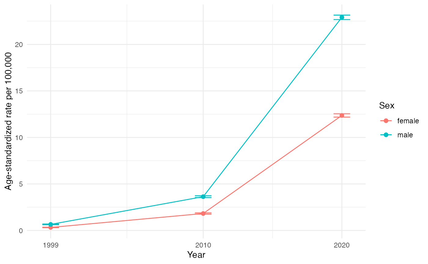

Line plot of age-standardized synthetic-opioid death rate per 100,000 against year for 1999, 2010, and 2020, with separate lines for males and females. Both lines rise steeply across the period, and the male line sits roughly twice as high as the female line in every year. Vertical bars show 95% confidence intervals.

Age-standardized synthetic-opioid (fentanyl-proxy) death rate per 100,000 by sex, illustrative data. Points are standardized rates and bars are 95% confidence intervals.

These counts are synthetic and illustrative only. A real analysis flags the restricted or public MCOD records exactly as shown above (see vignette("classifying-overdose-deaths")), aggregates them, and runs this same rate pipeline.

From records to a fentanyl flag

Aggregate to counts, then rate

Reading the result

See also