Trends in unspecified drug overdose deaths

Many drug-overdose death certificates never name the specific drug involved. That gap biases drug-specific trends – an apparent rise in one opioid can reflect improved toxicology and reporting specificity rather than a real increase in that drug. In ICD-10 data (1999 onward), the opioid deaths with no specific type are coded T40.6, “other and unspecified narcotics”, which narcan flags as other_op_present. This vignette measures the T40.6 share of opioid deaths by year, end to end, on small illustrative records; no restricted NCHS data are used and no chunk downloads anything.

library(narcan)

Illustrative records

The frame below is synthetic and illustrative. Each row is one death, coded in the ICD-10 convention – ucod is the underlying-cause code and f_records_all is the space-joined multiple-cause T-code string. Opioid deaths carry a poisoning ucod (X42, accidental poisoning by narcotics) plus one T40.x opioid code: heroin (T40.1), synthetic opioids such as fentanyl (T40.4), or the “other and unspecified” residual (T40.6). Two cocaine deaths per year (T40.5) are included so the opioid filter has something to remove. Counts are chosen so the T40.6 share falls as more deaths get a specific opioid type over time.

recipe <- tibble::tribble(
    ~year, ~ucod, ~f_records_all, ~n,
    1999L, "X42", "T401",         4L,   # heroin
    1999L, "X42", "T404",         2L,   # synthetic (e.g. fentanyl)
    1999L, "X42", "T406",         4L,   # other/unspecified opioid
    1999L, "X42", "T405",         2L,   # cocaine (non-opioid drug death)
    2005L, "X42", "T401",         5L,
    2005L, "X42", "T404",         3L,
    2005L, "X42", "T406",         4L,
    2005L, "X42", "T405",         2L,
    2012L, "X42", "T401",         6L,
    2012L, "X42", "T404",         6L,
    2012L, "X42", "T406",         3L,
    2012L, "X42", "T405",         2L,
    2019L, "X42", "T401",         8L,
    2019L, "X42", "T404",         9L,
    2019L, "X42", "T406",         3L,
    2019L, "X42", "T405",         2L
)
deaths <- recipe[rep(seq_len(nrow(recipe)), recipe$n),
                 c("year", "ucod", "f_records_all")]
rownames(deaths) <- NULL
nrow(deaths)
#> [1] 65

Walk the flags, one step at a time

Each flag keys on ucod plus f_records_all, and the ICD era is read from year, so run the pipeline one year at a time. Here is the 2012 slice through each step.

flag_drug_deaths() adds drug_death – for ICD-10 it is 1 when a qualifying poisoning ucod pairs with a drug T-code. All four 2012 record types qualify.

d12 <- deaths[deaths$year == 2012, ]
s1 <- flag_drug_deaths(d12, year = 2012)
head(s1)
#> # A tibble: 6 × 4
#>    year ucod  f_records_all drug_death
#>   <int> <chr> <chr>              <dbl>
#> 1  2012 X42   T401                   1
#> 2  2012 X42   T401                   1
#> 3  2012 X42   T401                   1
#> 4  2012 X42   T401                   1
#> 5  2012 X42   T401                   1
#> 6  2012 X42   T401                   1

flag_opioid_deaths() adds opioid_death, which additionally requires a T40.0-.4 or T40.6 opioid code. The three opioid rows stay 1; the cocaine death (T40.5) drops to 0.

s2 <- flag_opioid_deaths(s1, year = 2012)
unique(subset(s2, f_records_all %in% c("T401", "T406", "T405")))  # heroin, other/unspecified, cocaine
#> # A tibble: 3 × 5
#>    year ucod  f_records_all drug_death opioid_death
#>   <int> <chr> <chr>              <dbl>        <dbl>
#> 1  2012 X42   T401                   1            1
#> 2  2012 X42   T406                   1            1
#> 3  2012 X42   T405                   1            0

flag_opioid_types() adds the six specific-type columns, the ICD-9-era residual unspecified_op_present, and num_opioids. The T40.6 deaths land in other_op_present; unspecified_op_present stays 0 (see the closing note).

s3 <- flag_opioid_types(s2, year = 2012)
type_cols <- c("ucod", "f_records_all", "opioid_death", "heroin_present",
               "other_synth_present", "other_op_present",
               "unspecified_op_present", "num_opioids")
as.data.frame(unique(s3[s3$opioid_death == 1, type_cols]))
#>   ucod f_records_all opioid_death heroin_present other_synth_present
#> 1  X42          T401            1              1                   0
#> 2  X42          T404            1              0                   1
#> 3  X42          T406            1              0                   0
#>   other_op_present unspecified_op_present num_opioids
#> 1                0                      0           1
#> 2                0                      0           1
#> 3                1                      0           1

Apply the same three steps to every year, keep the opioid deaths, and take the mean of other_op_present per year – that mean is the T40.6 share.

flagged <- dplyr::bind_rows(lapply(split(deaths, deaths$year), function(d) {
    y <- d$year[1]
    d |>
        flag_drug_deaths(year = y) |>
        flag_opioid_deaths(year = y) |>
        flag_opioid_types(year = y)
}))

unspec <- flagged |>
    dplyr::filter(opioid_death == 1) |>
    dplyr::group_by(year) |>
    dplyr::summarize(
        opioid_deaths = dplyr::n(),
        t406_unspecified = sum(other_op_present),
        t406_share = round(mean(other_op_present), 3),
        .groups = "drop"
    )
unspec
#> # A tibble: 4 × 4
#>    year opioid_deaths t406_unspecified t406_share
#>   <int>         <int>            <dbl>      <dbl>
#> 1  1999            10                4      0.4  
#> 2  2005            12                4      0.333
#> 3  2012            15                3      0.2  
#> 4  2019            20                3      0.15

The T40.6 share falls from 0.40 in 1999 to 0.15 in 2019 – built into these illustrative counts, but the identical computation on real MCOD records recovers whatever trend the data actually hold.

library(ggplot2)

ggplot(unspec, aes(x = year, y = t406_share)) +
    geom_line() +
    geom_point() +
    labs(
        x = "Year",
        y = "T40.6 share of opioid deaths",
        title = "Unspecified-opioid-type (T40.6) share by year"
    )

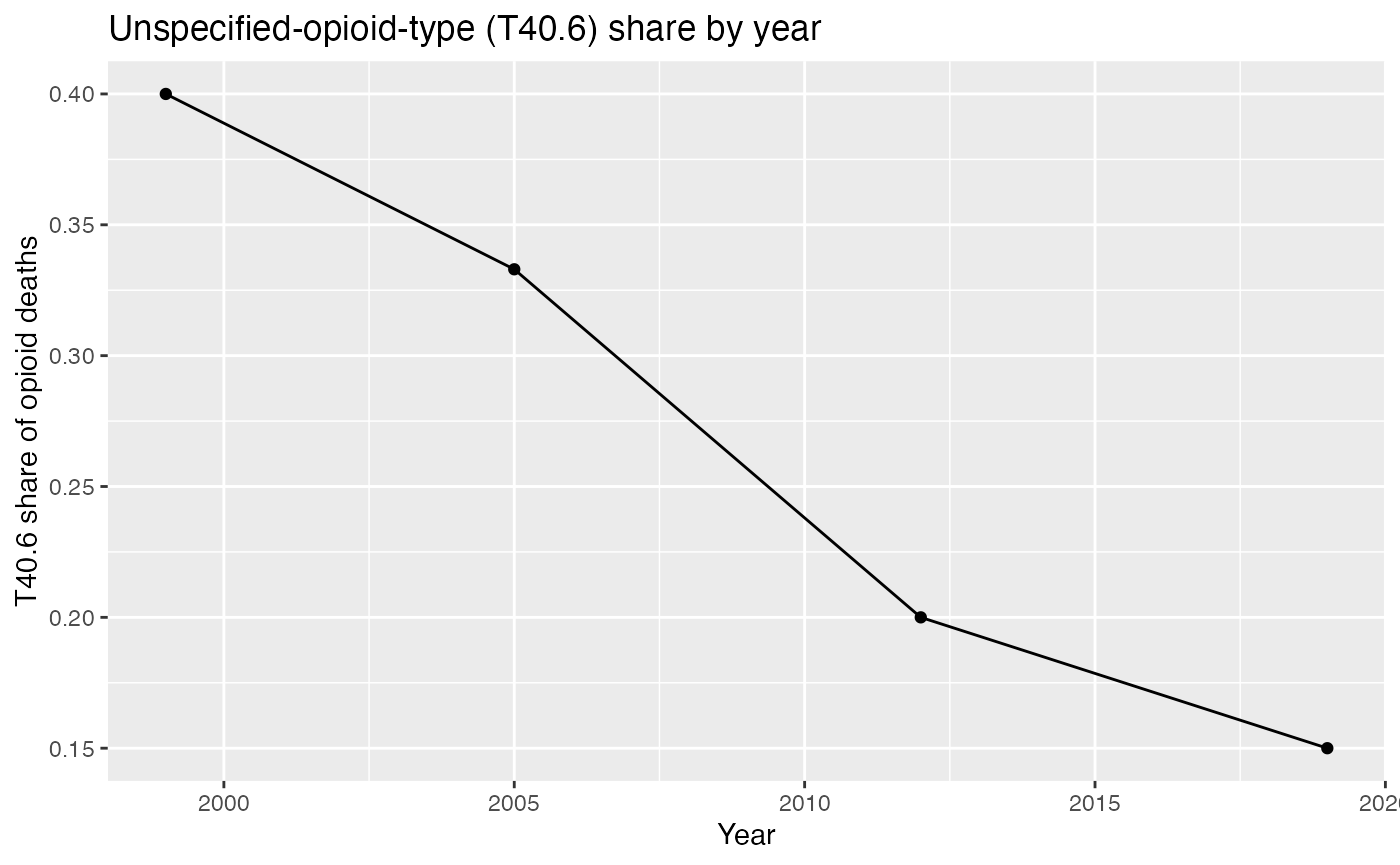
Line-and-point chart of the T40.6 (other and unspecified opioid) share of opioid deaths by year. The share falls from about 0.40 in 1999 to about 0.15 in 2019.

T40.6 (other/unspecified opioid) share of opioid deaths by year, computed from the illustrative records above.

Caveats

T40.6 is the standard ICD-10 proxy for an unspecified opioid, but the label is “other and unspecified narcotics”, so a T40.6 death is one where the specific opioid was not distinguished, not strictly one that is missing. This is the opioid type-unspecified share, not the broader problem of drug deaths with no specific drug coded at all, which spans non-opioid drugs too. narcan also carries unspecified_op_present, the ICD-9-era residual keyed to the generic opiate code 965.0; it is 0 by construction for years >= 1999 because ICD-10 folds the unspecified opioids into T40.6, which is exactly why the modern measure reads other_op_present instead. Some analysts redistribute T40.6 deaths across the known types before computing drug-specific rates; narcan gives you the raw flags so you can measure the unspecified share first and decide how to adjust for it yourself.

The unspecified share also varies markedly by jurisdiction, not only over time – some states (Pennsylvania is a persistent example) code a far higher fraction as unspecified than others (Buchanich et al. 2018; Ruhm 2018), and ISW7 notes the opioid purity of T40.6 itself varies by jurisdiction (it can occasionally capture non-opioid narcotics). A reassuring national decline can hide states where specificity stays poor, so check the share sub-nationally before trusting drug-specific rates there.

Illustrative records

Walk the flags, one step at a time

Unspecified (T40.6) share by year

Caveats

See also